CDS Pricing with the Merton Model

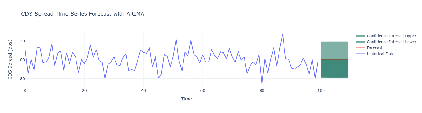
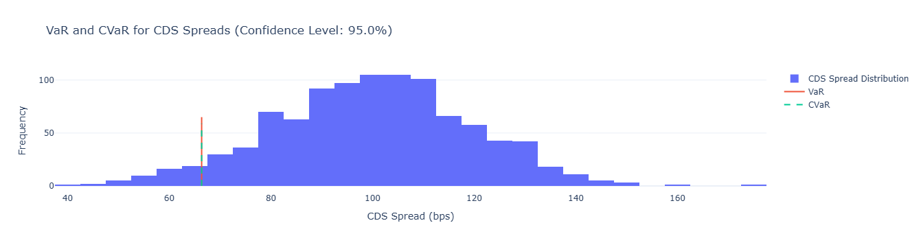
Monte Carlo simulation for CDS spread distribution and stress testing under changing risk factors.

Credit Default Swap (CDS) pricing can be linked to the probability of default (PD) implied by the Merton model. The model treats a firm’s equity as a call option on its assets with debt as the strike. Default occurs when asset values fall below debt obligations at maturity.

Monte Carlo Simulation

A Monte Carlo approach is used to estimate CDS spreads. Each simulation iteration generates one asset price path, computes distance-to-default, derives PD, and then maps it to spreads. This avoids redundant nested simulations.

Stress Testing

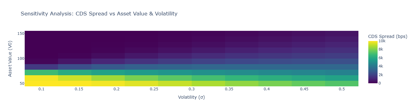
Stress tests allow us to evaluate CDS spreads under extreme but plausible market conditions. Factors such as volatility ($\sigma$), asset drift ($\mu$), debt level ($D$), and maturity ($T$) can be shocked to observe sensitivity in spreads.

Asset Dynamics (GBM)

Asset values follow a stochastic process:

\[ dS_t = r S_t \, dt + \sigma S_t \, dW_t \]

$S_t$: asset value at time $t$
$r$: risk-free rate
$\sigma$: asset volatility
$W_t$: standard Brownian motion

Probability of Default (PD)

Distance to Default (DD):

\[ \mathrm{DD} = \frac{\ln\!\left(\frac{V_0}{D}\right) + \left(r + \tfrac{1}{2}\sigma^2\right)T}{\sigma \sqrt{T}} \]

Default probability at maturity $T$:

\[ \mathrm{PD} = \Phi(-\mathrm{DD}) \]

CDS Spread (bps)

Given a recovery rate $R$ and probability of default $\mathrm{PD}$, an illustrative spread formula is:

\[ s = (1 - \mathrm{PD}) \times 10000 \]

Monte Carlo Simulation

The Monte Carlo estimator for CDS spread is:

\[ \hat{s}_{\mathrm{MC}} = \frac{1}{N}\sum_{i=1}^{N} \left[ \left(1 - \Phi\!\left( -\frac{\ln(S_i / D) + (r + \tfrac{1}{2}\sigma^2)T}{\sigma \sqrt{T}} \right)\right)\times 10000 \right] \]

Summary

Model defaults via Merton; compute PD from distance-to-default.
Estimate spreads through Monte Carlo using one path per iteration.
Stress test $\mu$, $\sigma$, $D$, and $T$ to gauge sensitivity.

Reference

Model defaults via Merton; CDS Pricing.